The purpose of Continuous Deployment is to increase Quality and Efficiency,
see e.g. The Software Revolution behind Linkedin’t Gushing Profits or read on
This posting presents an overview of Atbrox’ ongoing work on Automated Continuous Deployment. We develop in several languages depending on project or product, e.g. C/C++ (typically with SWIG combined with Python, or combined with Objective C), C# , Java (typically Hadoop/Mapreduce-related) and Objective-C (iOS). But most of our code is in Python (together with HTML/Javascript for frontends and APIs) and this posting will primarily show Python-centric continuous deployment with Jenkins (total flow) and also some more detail on the testing Tornado apps with Selenium.
Continuous Deployment of a Python-based Web Service / API
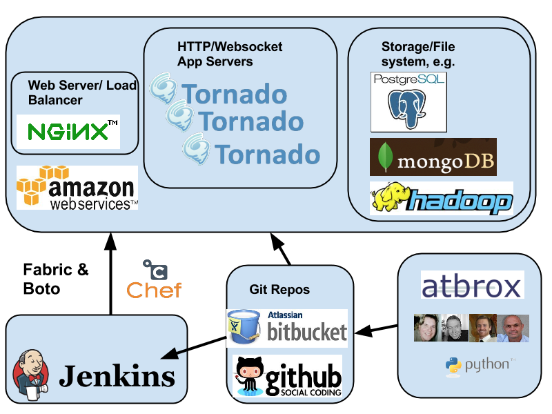
Many of the projects we develop involve creating a HTTP/REST or websocket API that generically said “does something with data” and has a corresponding UI in Javascript/HTML. The typical building stones of such a service is shown in the figure:
The flow is roughly as follows
- An Atbrox developer submits code into a git repo (e.g. Bitbucket.org or Github.com repo)
- Jenkins picks up the change (by notification from git or by polling)
- Tests are run, e.g. [sourcecode language=”python” wraplines=”false” collapse=”false”]
py.test -v –junitxml=result.xml –cov-report html –cov-report xml –cov .
[/sourcecode]
- Traditional Python unit tests
- Tornado web app asynchronous tests – http://www.tornadoweb.org/en/stable/testing.html
- Selenium UI Tests (e.g. with PhantomJS or xvfb/pyvirtualdisplay)
- Various metrics, e.g. test coverage, lines of code (sloccount), code duplication (PMD) and static analysis (e.g. pylint or pychecker)
- If tests and metrics are ok:
- provision cloud virtual machines (currently AWS EC2) if needed with fabric and boto, e.g. [sourcecode language=”python” wraplines=”false” collapse=”false”]
fab service launch
[/sourcecode]
- deploy to provisioned or existing machines with fabric and chef (solo), e.g.
[sourcecode language=”javascript” wraplines=”false” collapse=”false”]
fab service deploy
[/sourcecode]
- Fortunately Happy customer (and atbrox developer). Goto 1.
Example of selenium test of Tornado Web Apps with PhantomJS
Tornado is a python-based app server that supports Websocket and HTTP (it was originally developed by Bret Taylor while he was a FriendFeed). In addition to the python-based tornado apps you typically write a mix of javascript code and html templates for the frontend. The following example shows how to selenium tests for Tornado can be run:
Utility methods for starting a Tornado application and pick a port for it
[sourcecode language=”python” wraplines=”false” collapse=”false”]
import os
import tornado.ioloop
import tornado.httpserver
import multiprocessing
def create_process(port, queue, boot_function, application, name,
instance_number, service,
processor=multiprocessing):
p = processor.Process(target=boot_function,
args=(queue, port,
application, name,
instance_number, service))
p.start()
return p
def start_application_server(queue, port, application, name,
instance_number, service):
http_server = tornado.httpserver.HTTPServer(application)
http_server.listen(port)
actual_port = port
if port == 0: # special case, an available port is picked automatically
# only pick first! (for now)
assert len(http_server._sockets) > 0
for s in http_server._sockets:
actual_port = http_server._sockets[s].getsockname()[1]
break
pid = os.getpid()
ppid = os.getppid()
print "INTERNAL: actual_port = ", actual_port
info = {"name":name, "instance_number": instance_number,
"port":actual_port,
"pid":pid,
"ppid": ppid,
"service":service}
queue.put_nowait(info)
tornado.ioloop.IOLoop.instance().start()
[/sourcecode]
Example Tornado HTTP Application Class with an HTML form
[sourcecode language=”python” wraplines=”false” collapse=”false”]
# THE TORNADO CLASS TO TEST
class MainHandler(tornado.web.RequestHandler):
def get(self):
html = """
<html>
<head><title>form title</title></head>
<body>
<form name="input" action="http://localhost" method="post" id="formid">
Query: <input type="text" name="query" id="myquery">
<input type="submit" value="Submit" id="mybutton">
</form>
</body>
</html>
"""
self.write(html)
def post(self):
self.write("post returned")
[/sourcecode]
Selenium unit test for the above Tornado class
[sourcecode language=”python” wraplines=”false” collapse=”false”]
class MainHandlerTest(unittest.TestCase):
def setUp(self):
self.application = tornado.web.Application([
(r"/", MainHandler),
])
self.queue = multiprocessing.Queue()
self.server_process = create_process(0,self.queue,start_application_server,self.application,"mainapp", 123, "myservice")
self.driver = webdriver.PhantomJS(‘/usr/local/bin/phantomjs’)
def testFormSubmit(self):
data = self.queue.get()
URL = "http://localhost:%s" % (data[‘port’])
self.driver.get(‘http://localhost:%s’ % (data[‘port’]))
assert "form title" in self.driver.title
element = self.driver.find_element_by_id("formid")
# since port is dynamically assigned it needs to be updated with the port in order to work
self.driver.execute_script("document.getElementById(‘formid’).action=’http://localhost:%s’" % (data[‘port’]))
# send click to form and receive result??
self.driver.find_element_by_id("myquery").send_keys("a random query")
self.driver.find_element_by_id("mybutton").click()
assert ‘post returned’ in self.driver.page_source
def tearDown(self):
self.driver.quit()
self.server_process.terminate()
if __name__ == "__main__":
unittest.main(verbosity=2)
[/sourcecode]
Conclusion
The posting have given and overview of Atbrox’ (in-progress) Python-centric continuous deployment setup, with some more details how to do testing of Tornado web apps with Selenium. There are lots of inspirational and relatively recent articles and presentations about continuous deployment, in particular we recommend you to check out:
- Etsy’s slideshare about continuous deployment and delivery
- the Wired article about The Software Revolution Behind LinkedIn’s Gushing Profits
- Continuous Deployment at Quora
Please let us know if you have any comments or questions (comments to this blog post or mail to info@atbrox.com)
Best regards,
The Atbrox Team
Side note: We’re proponents and bullish of Python and it is inspirational to observe the trend that several major Internet/Mobile startups/companies are using it for their backend development, e.g. Instagram, Path, Quora, Pinterest, Reddit, Disqus, Mozilla and Dropbox. The largest python-based backends probably serve more traffic than 99.9% of the world’s web and mobile sites, and that is usually sufficient capability for most projects.