
Atbrox is startup providing technology and services for Search and Mapreduce/Hadoop. Our background is from from Google, IBM and Research.
Update 2010-June-17 Code for this posting is now on github –http://github.com/atbrox/Snabler
This posting gives an example of how to use Mapreduce, Python and Numpy to parallelize a linear machine learning classifier algorithm for Hadoop Streaming. It also discusses various hadoop/mapreduce-specific approaches how to potentially improve or extend the example.
1. Background
Classification is an everyday task, it is about selecting one out of several outcomes based on their features, e.g
- In recycling of garbage you select the bin based on the material, e.g. plastic, metal or organic.
- When purchasing you select the store from based e.g. on its reputation, prior experience, service, inventory and prices
Computational Classification – Supervised Machine Learning – is quite similar, but requires (relatively) well-formed input data combined with classification algorithms.
1.1 Examples of classification problems
- Finance/Insurance
- Classify investment opportunities as good or not e.g. based on industry/company metrics, portfolio diversity and currency risk.
- Classify credit card transactions as valid or invalid based e.g. location of transaction and credit card holder, date, amount, purchased item or service, history of transactions and similar transactions
- Biology/Medicine
- Classification of proteins into structural or functional classes
- Diagnostic classification, e.g. cancer tumours based on images
- Internet
- Document Classification and Ranking
- Malware classification, email/tweet/web spam classification
- Production Systems (e.g. in energy or petrochemical industries)
- Classify and detect situations (e.g. sweet spots or risk situations) based on realtime and historic data from sensors
1.2 Classification Algorithms
Classification algorithms comes in various types (e.g. linear, nonlinear, discriminative etc), see my prior postings Pragmatic Classification: The Very Basics and Pragmatic Classification of Classifiers.
Key takeaways about classifiers:
- There is no silver bullet classifier algorithm or feature extraction method.
- Classification algorithms tend to be computationally hard to train, this encourages using a parallel approach, in this case with Hadoop/Mapreduce.
2. Parallel Classification for Hadoop Streaming
The classifier described belongs to a familiy of classifiers which have in common that they can mathematically be described as Tikhonov Regularization with a Square loss function, this family includes Proximal SVM, Ridge Regression, Shrinkage Regression and Regularized Least-Squares Classification. (note: If you replace the Square Loss function with a Hinge-Loss function you get Support Vector Machine classification). The implemented classifier – proximal SVM – is from the paper Incremental Support Vector Machine Classification, referred to as the paper below.
2.1 training data
The classifier assumes numerical training data, where each class is either -1.0 og +1.0 (negative or positive class), and features are represented as vectors of positive floating point numbers. In the algorithm below are:
D - a matrix of training classes, e.g. [[-1.0, 1.0, 1.0, .. ]] A - a matrix with feature vectors, e.g. [[2.9, 3.3, 11.1, 2.4], .. ] e - a vector filled with ones, e.g [1.0, 1.0, .., 1.0] E = [A -e] mu = scalar constant # used to tune classifier D - a diagonal matrix with -1.0 or +1.0 values (depending on the class)2.2 the classifier algorithm
Training the classifier can be done with right side of the equation (13) from paper
(omega, gamma) = (I/mu + E.T*E).I*(E.T*D*e)Classification of an incoming feature vector x can then be done by calculating:
x.T*omega - gammawhich returns a number, and the sign of the number corresponds to the class, i.e. positive or negative.
2. Parallelization of the classifier with Hadoop Streaming and Python
Expression (16) in the paper has a nice property, it supports increments (and decrements), in the example there are 2 increments (and 2 decrements), but by induction there can be as many as you want:
(omega, gamma) = (I/mu + E_.T*E_1 + .. + E_i.T*E_i).I* (E_1.T*D_1*e + .. + E_i.T*D_i*e)where
E.T*E = E_1.T*E_1 + .. + E_i.T*E_iand
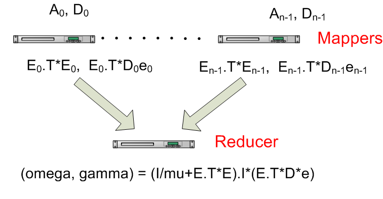
E.T*De = E_1.T*D_1*e + .. + E_i.T*D_i*eThis means that we can parallelize the calculation of E.T*E and E.T*De, by having Hadoop mappers calculate each of the elements of the sums in as in the Python map() code below (sent to reducers as tuples)
2.3 – the mapper
def map(key, value): # input key= class for one training example, e.g. "-1.0" classes = [float(item) for item in key.split(",")] # e.g. [-1.0] D = numpy.diag(classes) # input value = feature vector for one training example, e.g. "3.0, 7.0, 2.0" featurematrix = [float(item) for item in value.split(",")] A = numpy.matrix(featurematrix) # create matrix E and vector e e = numpy.matrix(numpy.ones(len(A)).reshape(len(A),1)) E = numpy.matrix(numpy.append(A,-e,axis=1)) # create a tuple with the values to be used by reducer # and encode it with base64 to avoid potential trouble with '\t' and '\n' used # as default separators in Hadoop Streaming producedvalue = base64.b64encode(pickle.dumps( (E.T*E, E.T*D*e) ) # note: a single constant key "producedkey" sends to only one reducer # somewhat "atypical" due to low degree of parallism on reducer side print "producedkey\t%s" % (producedvalue)2.4 – the Reducer
def reduce(key, values, mu=0.1): sumETE = None sumETDe = None # key isn't used, so ignoring it with _ (underscore). for _, value in values: # unpickle values ETE, ETDe = pickle.loads(base64.b64decode(value)) if sumETE == None: # create the I/mu with correct dimensions sumETE = numpy.matrix(numpy.eye(ETE.shape[1])/mu) sumETE += ETE if sumETDe == None: # create sumETDe with correct dimensions sumETDe = ETDe else: sumETDe += ETDe # note: omega = result[:-1] and gamma = result[-1] # but printing entire vector as output result = sumETE.I*sumETDe print "%s\t%s" % (key, str(result.tolist()))2.5 – Mapper and Reducer Utility Code
Code used to run map() and reduce() methods, inspired by iterator/generator approach from this mapreduce tutorial.
def read_input(file, separator="\t"): for line in file: yield line.rstrip().split(separator)def run_mapper(map, separator="\t"): data = read_input(sys.stdin,separator) for (key,value) in data: map(key,value)def run_reducer(reduce,separator="\t"): data = read_input(sys.stdin, separator) for key, values in groupby(data, itemgetter(0)): reduce(key, values)3. Finished?
Assume your running time goes through the roof even with the above parallel approach, what to do?
3.1 Mapper Increment Size really makes a difference!
Since there is only 1 reducer in the presented implementation, it is useful to let mappers do most of the job. The size of the (increment) matrices – E.T*E and E.T*D*e given as input to the reducer is independent of number of training data, but dependent on the number of classification features. The workload on the reducer is also dependent on the number of matrices received by the mappes (i.e. increment size), e.g. if you have a 1000 mappers having one billion examples with 100 features each, the reducer would need to do a sum of one trillion 101×101 matrices and one trillion 101×1 vectors if the mapper sent one matrix pair per training example, but if each mapper only sent one pair of E.T*E and E.T*D*e representing all the mappers billion training examples the reducer would only need to summarize 1000 matrix pairs.
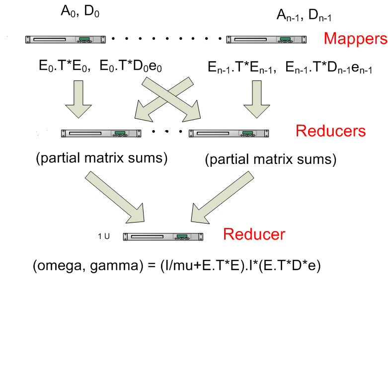
3.2 Avoid stressing the reducer
Add more (intermediate) reducers (combiners) that calculates partial sums of matrices. In the case of many small increments (and correspondingly many matrices) it can be useful to add an intermediate step that (in parallel) calculates sums of E.T*E and E.T*D*e before sending the sums to the final reducer, this means that the final reducer gets fewer matrices to summarize before calculating the final answer, see figure below.
3.3 Parallelize (or replace) the matrix inversion in the reduction step
If someone comes along with a training data set with a very high feature-dimension (e.g. recommender systems, bioinformatics or text classification), the matrix inversion in the reducer can become a real bottleneck since such algorithms typically are O(n^3) (and lower bound of Omega(n^2 lg n)), where n is the number of features. A solution to this can be to use or develop hadoop/mapreduce-based parallel matrix inversion, e.g. Apache Hama, or don’t invert the matrix...
3.4 Feature Dimensionality Reduction
Another approach when having training data with high feature-dimension could be to reduce feature-dimensionality, for more info check out Latent Semantic Indexing (and Analysis), Singular Value Decomposition or t-Distributed Stochastic Neighbor Embedding
3.5 Reduce IO between mappers and reducers with compression
Twitter presented using LZO compression (on the Cloudera blog) to speed up Hadoop. Inspired by this one could in the case of high feature dimension, i.e. large E.T*E and E.T*D*e matrices, compress the output in the mapper and decompress in the reducer by replacing base64encoding/decoding and pickling above with:
producedvalue = base64.b64encode(lzo.compress(pickle.dumps( (E.T*E, E.T*D*e) ), level=1)and
ETE, ETDe = pickle.loads(lzo.decompress(base64.b64decode(value)))3.6 Do more work with approximately the same computing resources
The D matrix above represents binary classification with a value of +1 or -1 representing each class. It is quite common to have classification problems with more than 2 classes. Supporting multiple classes is usually done by training by several classifiers, either 1-against-all (1 classifier trained per class) or 1-against-1 (1 classifier trained per unique pair of classes), and the run a tournament of them against each other and pick the most confident. In the case of 1-against-all classification the mapper could probably send multiple E.T*D_c*e – with one D_c per class and keep the same E.T*E, the reducer would then need to calculate (I/mu + E.TE).I once and independently multiply with several E.T*D_c*e sums to create a set of (omega,gamma) classifiers. For 1-against-1 classification it becomes somewhat more complicated, because it involves creating several E matrices since in the 1-against-1 case only the rows in E where the 2 classes competing occur are relevant.
4. Code
(Early) Python code of the algorithm presented above can be found at http://github.com/atbrox/Snabler (open source with Apache Licence). Please let me know if you want to contribute to the project, e.g. from mapreduce and hadoop algorithms in academic papers.
5. More resources about machine learning with Hadoop/Mapreduce?
- Apache Mahout – active project that implements (in Java) several machine learning algorithms (also unsupervised machine learning, i.e. clustering)
- Good paper about machine learning algorithms with mapreduce – http://www.cs.stanford.edu/people/ang//papers/nips06-mapreducemulticore.pdf
Best regards,
Amund Tveit, co-founder of Atbrox
Pingback: Quora
Pingback: Quora
Pingback: Data Mining on Distributed System – the cosmos
Pingback: Brief Introduction to Hadoop and its ecosystem « FLOW-HEART AND ALGO-RYTHMS
Pingback: Mapreduce & Hadoop Algorithms in Academic Papers (3rd update) | Luciuz's Homepage
Pingback: Python:Are there any distributed machine learning libraries for using Python with Hadoop? [closed] – IT Sprite
Pingback: Python:Efficient outer product in python – IT Sprite
Pingback: Getting Started with Code: A List of Tutorials and Resources